How the Model works?
The Basic Model
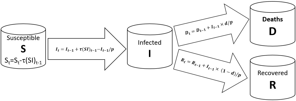
Legend
\begin{align} S & = \text{Susceptible population } \\ I & = \text{Infected}\\ D & = \text{Deaths } \\ R & = \text{Recovered} \\ \rho & = \text{infectiousness/communicability period} \\ \delta & = \text{The death rate} \\ t & = \text{Time period t} \\ \tau & = \text{The rate of transmission} \\ & = \frac{(I_{t} - I_{t-1})}{(SI)_{t-1}} \\ & = \frac{\Delta I_{t}}{(SI)_{t-1}} \end{align}
The Basic Model
Defining the rate of infectiousness R0 on day zero as
\( RO = \frac{I_{t=0} - I_{t-1}}{I_{t-1}} \times \rho = \frac{\Delta I_{t=-1}}{I_{t=-1}} \times \rho \)
then the transmission rate on day zero can be alternatively written as
\( \tau_{t=0} = \frac{RO_{t=0}}{\rho S_{t-1}}\)
The public health intervention, which lets the user define the day on which R0 becomes zero, \( t_{RO=0}\), is linearly reduced as
\( \tau_{t} = \frac{RO_{t=0}}{\rho S_{t-1}} - \frac{\frac{RO_{t=0}}{\rho S_{t-1}}}{t_{RO=0}} \times t \ \forall \ t < t_{RO=0}, 0 \ otherwise\)
Confidence Intervals of Projections
The upper and lower limit of the projections were calculated on the estimated transmission rates using the country specific data
for \(I_{t=-10} \) to \(I_{t=0} \), specifically
\(se(\tau)=\frac{\frac{\sum_{t=-10}^{0} (\tau_{t} - \bar{\tau})^2}{9}}{\sqrt{10}} \)
where
\( \bar{\tau} = \frac{\sum_{t=-10}^{0} \tau_{t}}{10}\)
Moreover, we assumed that the susceptible population during \( [-10 \leq t \leq 0]\) is equal to the respective country’s 2019 population
(Source: UN Population Prospects).
The upper and lower limits for \( \tau_{t=0}\) are then \( \tau_{t=0} \pm 1.96 \times se(\tau) \).